I had some reading hours about how to approach our particular problem. Anomaly detection is apparently called ‘outlier detection’ in scientific context, and it is not a trivial task at all. From a data-analysis perspective, anomalies in data are the ones that attract interest. This means that finding and spotting anomalies is a valuable and an important task.
What is an anomaly?
An anomaly is the difference between a measurement and a mean or a model prediction.
This is one of the wikipedia definitions. To put it bluntly: it is an event that stands out from the normal. This is simple enough, but when applied to a context we get to ask: what is normal? There are other considerations as well: what if an anomaly is purposedly tailored to look like a normal event? Also if the context changes fundamentally, everything looks weird from the earlier normal perspective.
One of the problems with anomaly (or outlier) detection is that the anomalies are often rare and obscure. There is no data available. We mostly only know and prefer the ‘normal’ conditions. The classification task is difficult if we can’t distinguish the freaks from the normals. Sounds quite like real life. Luckily we are not classifying people here but logs. Not as sawing industry does but as log entries in log files where computer events are recorded.
Simple ML model: Autoencoder
A neural network autoencoder is like zip-unzip process: it learns to reproduce it’s own data squeezing it through fewer parameters than it had originally. We want to make our detector work first on a simple level and an autoencoder fits this task. We are going to feed an autoencoding network with normal log data, and then compare an anomalous log line to the learned normal conditions.
Being an unsupervised task, the validation data with autoencoder is it’s own data, so it is relatively fast to train. With this technique, the machine learning model learns relations between the inputs.
The inputs are the individual Apache log items, and we have to employ a couple of methods to deal and process with them so they are usable in a neural network.
A fresh drawing
Our supervisor Tero Karvinen who gave us the original idea to the project tipped us on a meeting about a video, where a representative of Stripe (an online payment processing company) gives a talk on their machine learning usage in fraud detection. I found some other interesting news items about how Stripe collects this data. Touchy subject…
Despite the news, the talk on the subject is really good, on the point and professional. At one point Ms. Pamela Vagata presents a model graph:
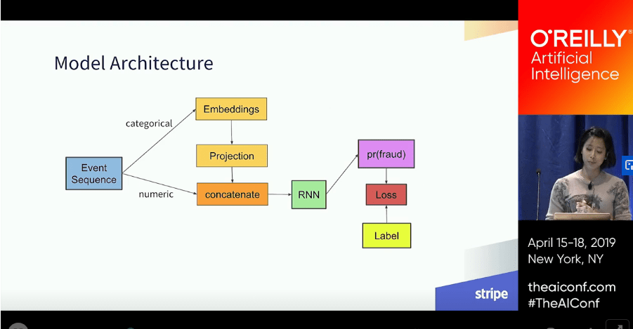
I don’t know, maybe I just wanted to see the similarities, but I got this strong feeling we’re on the right track. Obviously the model Stripe is using is more complex, and deals with huge amounts of data. She talks about categorizing the event sequences, which was really interesting concept, using LSTM’s (we’re not there yet), and quite a lot about similar problems we are facing.
Inspired by this, I refined and rethought the upcoming model:
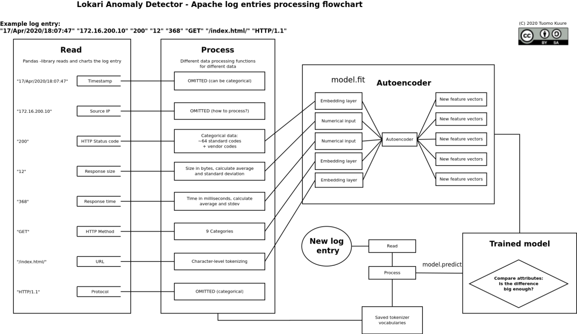
Embedding layers
Embedding layers can be used as categorical data can be processed with them. Thus the relations between HTTP status codes and client requested methods can also be dealt with these. Word embeddings are usually related to natural language processing, but categorical data’s cardinality can be reduced by embedding it. Cardinality refers to the number of categories in the set, and HTTP status codes are numerous. In reality we only see maybe 10 of them.
URL (and query), TF-IDF
At the moment this piece of text is handled per character. There are couple of choices, and the first trained model (untested as of yet) just converts the text into arrays of integers. Quite like antique cryptography did.
Another option we have to explore is to use tf-idf tokenizer. It performed best on the first demo. Tf-idf stands for term-frequency inverse-document-frequency. It gives a numerical value of how important a character is in that particular position of the text line. For example, a snippet from tfidf-converting url queries:
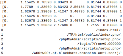
We can see that the slash as the first letter gets zero value. The dataset here is small, so the rest of the data is not that good an estimate.
The loss function
As usual with machine learning models, it boils down to an optimization problem, and a loss function is chosen, and is used to measure how well the model has been trained. I don’t get any deeper into this, as it is a complex subject, and there are tons of articles around explaining it. We are looking for small values.
The first version of the autoencoder today had really high losses, and they jumped erratically all around. I’m sorry I haven’t gotten into plotting all this. Graphics would definetely look better than these abysmally tiny numerical tables:

We are looking for loss values closing on zeroes, and on the outputs of ‘byte’ and ‘rtime’ they were much higher than expected. These were indeed 2 numbers that were not processed in any way as of yet.
Zscore
Statistics for the win! In Jeff Heaton’s Deep Learning course a statistical method was introduced to sort of compress the values. Given that we have the whole population at our hands, we can count the mean (average) and standard deviation for the said set.
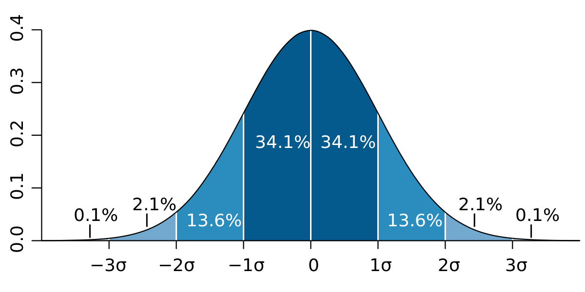
Standard score, or zscore then normalizes the deviation, so instead all the response times and sizes are given an relative value within the normal distribution. As we all love and know throughout our statistics and confidence levels, the result of this operation is, that ~95% of the values are within +2 and -2.
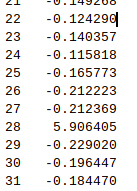
These are response times recalculated as standard score. That 5.9 is definetely off! Joni told me he used burp suite to delay the client responses to his test servers by a good margin.
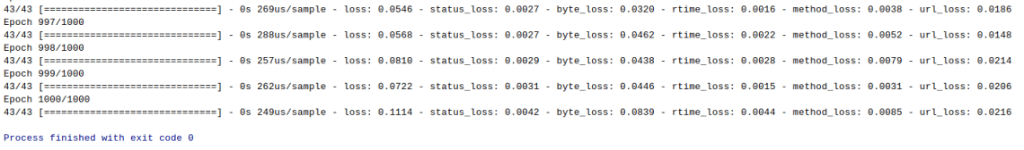
The results? I did this to both 2 numerical datas, and the loss value got quite low indeed:
Next phase
Next week we can start testing and validating the model. This is arguably the best part, as we get to stare at numbers dancing on the screen 😀
Sources
Here are some source links from my memos and bookmarks that have proven useful:
https://towardsdatascience.com/an-overview-of-categorical-input-handling-for-neural-networks-c172ba552dee
https://towardsdatascience.com/neural-network-embeddings-explained-4d028e6f0526
https://www.fast.ai/2018/04/29/categorical-embeddings/
https://stackoverflow.com/questions/53417537/keras-initialize-large-embeddings-layer-with-pretrained-embeddings
https://github.com/yzhao062/anomaly-detection-resources
https://www.pyimagesearch.com/2018/06/04/keras-multiple-outputs-and-multiple-losses/
https://medium.com/datadriveninvestor/unsupervised-outlier-detection-in-text-corpus-using-deep-learning-41d4284a04c8
